Section 1: Review of Grade 11 Physics
Section Learning Outcomes:
Section Key Terms:
Bored Already? Press the buttons to dive into applications!
Lesson 1: Review of Displacement, Velocity, and Acceleration in 1D and 2D
Distance and Displacement in 1D and 2D
Unless you have flown in an airplane, you have probably never traveled faster than 150 mph. Can you imagine travelling in a train that goes over 300 mph? Despite the high speed, the people riding in this train may not notice that they are moving at all unless they look out the window! This is because motion, even motion at 300 mph, is relative to the observer.
Our study of physics opens with - the study of motion without considering its causes. Objects are in motion everywhere you look. Everything from a football game to a race car driving around a corner involves motion. When you are resting, your heart moves blood through your veins. Even in inanimate objects, atoms are always moving.
How do you know something is moving? The location of an object at any particular time is its . More precisely, you need to specify its position relative to a convenient reference frame. Earth is often used as a reference frame, and we often describe the position of an object as it relates to stationary objects in that reference frame. For example, a rocket launch would be described in terms of the position of the rocket with respect to Earth as a whole, while a professor's position could be described in terms of where he or she is in relation to the nearby white board. In other cases, we use reference frames that are not stationary but are in motion relative to Earth. To describe the position of a person in an airplane, for example, we use the airplane, not Earth, as the reference frame. Thus, you can only know how fast and in what direction an object's position is changing against a background of something else that is either not moving or moving with a known speed and direction. The reference frame is the coordinate system from which the positions of objects are described.
As we study the motion of objects, we must first be able to describe the object's position. Imagine you are going for a walk in your neighbourhood. You start at your house, walk around the block, and end up at your friend's house. The you covered is the total length of the path you walked.

Figure 1: A person walking around their neighbourhood.
Physicists use variables to represent terms. We will use d to represent the person's position. We will use a subscript to differentiate between the initial position, d0, and the final position, df. Throughout this module there will be scalars and vectors which will be either italicized or bolded and italicized (or marked with an arrow), respectively.
We often want to be more precise when we talk about position. The description of an object's motion often includes more than just the distance it moves. For instance, if it is a three kilometer walk to your friend's house, the distance traveled is 3 kilometers. After spending time with your friend and walk back home, you will have traveled a total distance of 6 kilometers. You will end up in the same starting position in space.
Figure 2: A person walking to their friend's house and back.
The net change in position of an object is its . The Greek letter delta, Δ, means change in. If you are describing only your walk to your friend's house, then the distance traveled and the displacement are the same - 3 kilometers. When you are describing the entire round trip, distance and displacement are different. When you describe distance, you only include the , the size or amount, of the distance traveled. However, when you describe the displacement, you take into account both the magnitude of the change in position and the direction of movement.
In our previous example, you traveled a total of 6 kilometers, but you only walked three of those kilometers forward toward your friend's house and three of those kilometers back in the opposite direction. If we ascribe the forward direction a positive (+) and the opposite direction a negative (-), then the two quantities will cancel each other out when added together.
A quantity, such as distance, that has magnitude (i.e., how big or how much) but does not take into account direction is called a . A quantity, such as displacement, that has both magnitude and direction is called a .
Speed and Velocity in 1D and 2D
There is more to motion than distance and displacement. Questions such as, "How long does a foot race take?" and "What was the runner's speed?" cannot be answered without an understanding of other concepts. A description of how fast or slow an object moves is its and it is the rate at which an object changes its location. Like distance, speed and time are scalars because it has a magnitude but not a direction. Because speed is a rate, it depends on the time interval of motion. The elapsed time or change in time, Δt, of motion is the difference between the ending time and the beginning time
The International System of Units, internationally known by the abbreviation SI (for Système International), defines the second (s) as the unit of time and meters per second (m/s) for speed, but sometimes kilometers per hour (km/h), miles per hour (mph) or other unites of speed are used.
In racing, the starting lineup is determined by qualifying time trials in which the average speeds of the racers are compared. Each racer must cover the same distance around the track, and the racer with the shortest time gets pole (first) position. During some parts of the qualifying trials, other racers may have achieved a high , the speed at a particular instant, but the winner has the greatest average speed.
, vav, is the total distance traveled, d, divide by the total time of travel, Δt, or in equation form
Suppose a race is happening at a velodrome with a 250 meters circumference. If the fastest racer took 20 seconds to complete a lap, their average speed for the lap would be

Figure 3: Team Canada cyclists racing around a velodrome at the Olympics.
Now let's consider the scenario where a sprinter runs 100 meters towards the east and takes 11 seconds to do so. In this case, we have both the distance traveled and the direction, thus we have a vector quantity. The vector version of speed is and it describes the speed and direction of an object.
As with speed, it is useful to describe the over a time period. It is also useful to describe the , the velocity at a specific moment. The average velocity of an object like the sprinter is the displacement divided by the time over which the displacement occur, or in equation form
Velocity, like speed, has SI units of meters per second (m/s), but because it is a vector, you must also include a direction. It is important to keep in mind that the average speed is not the same thing as the average velocity without its direction. Like we saw with displacement and distance, changes in direction over a time interval have a bigger effect on speed and velocity.
Earlier, we talked about how the distance traveled can be different than the magnitude of displacement. In the same way, speed can be different than the magnitude of velocity. For example, you drive to a store and return home in half an hour. If your car's odometer shows the total distance traveled was 6 km, then your average speed was 12 km/h. Your average velocity, however, was zero because your displacement for the round trip is zero.
Acceleration in 1D and 2D
You may have heard the term accelerator, referring to the gas pedal in a car. When the gas pedal is pushed down, the flow of gasoline to the engine increases, which increases the car's velocity. Pushing on the gas pedal results in acceleration because the velocity of the car increases, and acceleration is defined as a change in velocity. You need two quantities to define velocity: a speed and a direction. Changing either of these quantities, or both together, changes the velocity. You may be surprised to learn that pushing on the brake pedal or turning the steering wheel also causes acceleration. The first reduces the speed and so changes the velocity, and the second changes the direction and also changes the velocity.
In fact, any change in velocity - whether positive, negative, directional, or any combination of these - is called an in physics. Acceleration is the change in velocity divided by a period of time during which the change occurs. The SI units of velocity are m/s and the SI units for time are s, so the SI units for acceleration are m/s2.
The of object is given by
Average acceleration is distinguished from , which is acceleration at a specific instant in time. The magnitude of acceleration is often not constant over time. For example, runners in a race accelerate at a greater rate in the first second of a race than during the following seconds. You do not need to know all the instantaneous accelerations at all times to calculate average acceleration. All you need to know is the change in velocity (i.e., the final velocity minus the initial velocity) and the change in time (i.e., the final time minus the initial time).
Keep in mind that although acceleration points in the same direction as the change in velocity, it is not always in the direction of the velocity itself. When an object slows down, its acceleration is opposite to the direction of its velocity. In everyday language, this is called deceleration; but in physics, it is acceleration - whose direction happens to be opposite that of the velocity. For now, let us assume that motion to the right along the x-axis is positive and motion to the left is negative.
Figure 6: Graphic showing positive and negative acceleration.
The defining equation for average acceleration, does not include displacement. As you will see soon, displacement can be found by determining the area under the line on a velocity-time graph. We can combine this observation with the defining equation for average acceleration to derive other equations useful in analyzing motion with constant acceleration. When acceleration is constant, a=aav, so we use the symbol a to represent the acceleration.
The area beneath the line in a velocity-time graph is the area of a trapezoid, Δd=1/2(vf+vi)Δt. This equation, without the variable a, can be combined with the defining equation for average acceleration to derive three other equations, each of which involves four of the five possible variables that are associated with constant acceleration. For example, to derive the equation in which Δt is eliminated, we omit the vector notation; this allows us to avoid the mathematical problem that would occur if we multiplied two vectors. We can now rearrange the defining equation to get Δt, which we can substitute to solve for Δd:
In a similar way, substitution can be used to derive the final two equations in which vf and vi are eliminated. The resulting five equations for constant acceleration are known as the kinematic equations and are presented as follows:
Constant Acceleration Problem-Solving Steps
While no single step-by-step method works for every problem, the following general procedures facilitate problem solving and make the answers more meaningful. A certain amount of creativity and insight are required as well.
- 1. Examine the situation to determine which physical principles are involved. It is vital to draw a simple sketch at the outset and to decide which direction is positive and note that on your sketch.
- 2. Identify the knowns: Make a list of what information is given or can be inferred from the problem statement. Remember, not all given information will be in the form of a number with units in the problem. If something starts from rest, we know the initial velocity is zero. If something stops, we know the final velocity is zero.
- 3. Identify the unknowns: Decide exactly what needs to be determined in the problem.
- 4. Find an equation or set of equations that can help you solve the problem. Your list of knowns and unknowns can help here. For example, if time is not needed or not given, then the fourth kinematic equation, which does not include time, could be useful.
- 5. Insert the knowns along with their units into the appropriate equation and obtain numerical solutions complete with units. This step produces the numerical answer; it also provides a check on units that can help you find errors. If the units of the answer are incorrect, then an error has been made.
- 6. Check the answer to see if it is reasonable: Does it make sense? This final step is extremely important because the goal of physics is to accurately describe nature. To see if the answer is reasonable, check its magnitude, its sign, and its units. Are the significant figures correct?
To solve a constant acceleration problem you should:
- 1. Determine the knowns and unknowns.
- 2. Find an equation that expresses the unknown in terms of the knowns. More than one unknown means more than one equation is needed.
- 3. Solve the equation or equations.
- 4. Be sure units and significant figures are correct.
- 5. Check whether the answer is reasonable.
Position, Velocity, and Acceleration Graphs
A graph, like a picture, is worth a thousand words. Graphs not only contain numerical information, they also reveal relationships between physical quantities. Graphs in this text have perpendicular axes, one horizontal and the other vertical. When two physical quantities are plotted against each other, the horizontal axis is usually the , and the vertical axis is the . In algebra, you would have referred to the horizontal axis as the x-axis and the vertical axis as the y-axis.
Consider a marathon runner moving along a straight road with a constant velocity of 5.5 m/s [S] for 3.0 minutes. At the start of the motion (i.e., at t=0), the initial position is d=0. The corresponding position-time data is shown in table 1 and the corresponding position-time graph is shown in Figure 10. Notice that for constant velocity motion, the position-time graph is a straight line.
Figure 10: Position-time graph of the runner's motion.
| Time t (s) | Position d (m) |
|---|---|
| 0 | 0 |
| 2 | 15 |
| 4 | 30 |
| 6 | 45 |
| 8 | 60 |
| 10 | 75 |
| 12 | 90 |
Table 1: Position-time data of the runner's motion.
Since the line on the position-time graph has a constant slope, we can calculate the slope, which it is the ratio of the change in the quantity on the vertical axis to the corresponding change in the quantity on the horizontal axis. Thus, the slope of the line on the position-time graph from t=0.0 s to t=12 s is
This value would be the same no matter which part of the line we used to calculate the slope. It is apparent that for constant velocity motion, the average velocity is equal to the instantaneous velocity at any particular time and that both are equal to the slope of the line on the position-time graph. Figure 11 is the corresponding velocity-time graph of the runner's motion.
Figure 11: Velocity-time graph of the runner's motion.
Now let's turn to graphs of motion with changing instantaneous velocity. This type of motion, often called nonlinear motion, involves a change of direction, a change in speed, or both. Consider, for example, a car starting from rest and speeding up, as in Table 2 and Figure 12.
Figure 12: Position-time graph of nonlinear motion.
| Time t (s) | Position d (m) |
|---|---|
| 0 | 0 |
| 1 | 1 |
| 2 | 4 |
| 3 | 9 |
| 4 | 16 |
Table 2: Position-time data of the nonlinear motion.
Since the slope of the line on the position-time graph is gradually increasing, the velocity is also gradually increasing. To find the slope of a curved line at a particular instant, we draw a straight line touching - but not cutting - the curve at that point. This straight line is called a to the curve. The slope of the tangent to a curve on a position-time graph is the instantaneous velocity.
Figure 13 shows the tangent drawn at 2.0 s for the motion of the car. The broken lines in the diagram show the average velocities between t=2.0 s and later times. For example, from t=2.0 s to t=8.0 s, Δt=6.0 s and the average velocity is the slope of line A. From t=2.0 s to t=6.0 s, Δt=4.0 s and the average velocity is the slope of line B, and so on. Notice that as Δt becomes smaller, the slopes of the lines get closer to the slope of the tangent at t=2.0 s (i.e., they get closer to the instantaneous velocity, v). Thus, we can define the instantaneous velocity as
Figure 13: Position-time graph of nonlinear motion showing the different slopes of lines.
When there is nonlinear motion, the velocity-time graph can be made based on the different slopes of the position-time graphs, shown in figure 14, with the corresponding velocity-time data shown in table 3. Since the velocity change over time, we now have an acceleration and we can draw an acceleration-time graph, shown in figure 15.
Figure 14: Velocity-time graph of nonlinear motion.
| Time t (s) | Velocity v (m/s) |
|---|---|
| 0 | 1.0 |
| 1 | 1.5 |
| 2 | 2.0 |
| 3 | 2.5 |
| 4 | 3.0 |
Table 3: Velocity-time data of the nonlinear motion.
Figure 15: Acceleration-time graph of nonlinear motion.
Lesson 2: Projectile Motion
Position, Velocity, and Acceleration Graphs
Imagine a snowboarder launching off a ramp on a snow-covered slope. Once the snowboarder leaves the ramp, they are subject to the forces of gravity and their initial velocity, as seen in figure 17. The motion can be divide into two independent components: horizontal motion and vertical motion.
Figure 17: Graphic of a snowboarder leaving the ramp and the forces acting on him and of the projectile motion.
In the absence of air resistance, the horizontal motion of the snowboarder is not affected by gravity. This means that the snowboarder will continue to move horizontally with a constant velocity throughout the entire motion. For example, if the snowboarder has an initial horizontal velocity of 10 m/s, that velocity will remain constant as long as no external forces (such as air resistance or wind) act upon them. Therefore, the snowboarder will travel a certain horizontal distance during the entire flight, called the .
In contrast to the horizontal motion, the vertical motion of the snowboarder is influenced by gravity. After leaving the ramp, the snowboarder will experience an initial vertical velocity and the downward force of gravity. As the snowboarder ascends, the vertical velocity decreases due to the opposing force of gravity. At the highest point of the jump, called the , the vertical velocity momentarily becomes zero. As the snowboarder descends, the vertical velocity increases in the downward direction due to the acceleration caused by gravity.
Throughout the entire motion, the snowboarder’s vertical position changes, resulting in a curved known as a parabola. The shape of the parabolic path depends on the initial launch angle, initial velocity, and the acceleration due to gravity. This type of motion is known as and refers to the motion of an object that is launched into the air and moves under the influence of gravity alone.
In projectile motion problems, we’ll call the horizontal axis the x-axis and the vertical axis the y-axis. For notation, d is the total displacement, and x and y are its components along the horizontal and vertical axes. As usual, we use velocity, acceleration, and displacement to describe motion. We must also find the components of these variables along the x- and y-axes. The components of acceleration are then very simple ay=-g=-9.81m/s2. Note that this definition defines the upwards direction as positive. Because gravity is vertical, ax=0. Both accelerations are constant, so we can use the kinematic equations:
Solving Problems Involving Projectile Motion
The following steps are used to analyze projectile motion:
- 1. Separate the motion into horizontal and vertical components along the x- and y-axes. These axes are perpendicular, so Ax=Acosθ and Ay=Asinθ are used. The magnitudes of the displacement s along x- and y-axes are called x and y. The magnitudes of the components of the velocity v are vx=vcosθ and vy=vsinθ, where v is the magnitude of the velocity and θ is its direction. Initial values are denoted with a subscript 0.
- 2. Treat the motion as two independent one-dimensional motions, one horizontal and the other vertical. The kinematic equations for horizontal and vertical motion take the following forms
- a. Horizontal motion (ax=0): x=x0+vx t and vx=v0x=vx=velocity is a constant
- b. Velocity motion (assuming positive is up, ay=-g=-9.81m/s2): y=y0+1/2 (v0y+vy)t, vy=v0y-gt, y=y0+v0y t-1/2 gt2, and vy2=v0y2-2g(y-y0)
- 3. Solve for the unknowns in the two separate motions (one horizontal and one vertical). Note that the only common variable between the motions is time t. The problem solving procedures here are the same as for one-dimensional kinematics.
- 4. Recombine the two motions to find the total displacement s and velocity v. We can use the analytical method of vector addition, which uses and to find the magnitude and direction of the total displacement and velocity.
For problems of projectile motion, it is important to set up a coordinate system. The first step is to choose an initial position for x and y. Usually, it is simplest to set the initial position of the object so that x0=0 and y0=0.
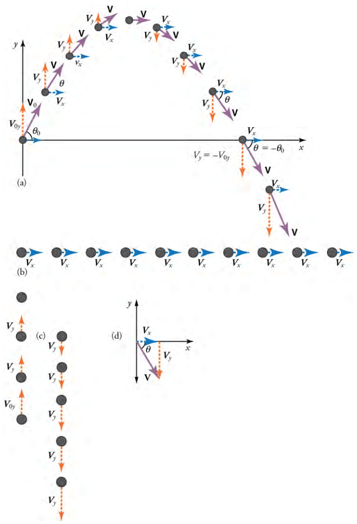
Figure 18: (a) We analyze two-dimensional projectile motion by breaking it into two independent one-dimensional motions along the vertical and horizontal axes. (b) The horizontal motion is simple because a_x=0 and v_x is thus constant. (c) The velocity in the vertical direction begins to decrease as the object rises; at its highest point, the vertical velocity is zero. As the object falls towards the Earth again, the vertical velocity increases again in magnitude but points in the opposite direction to the initial vertical velocity. (d) The x- and y-motions are recombined to give the total velocity at any given point on the trajectory (Open Stax High School Physics, 2022).
Lesson 3: Introduction to Frames of Reference and Relative Motion
Frames of Reference and Relative Velocity
Air shows provide elements of both excitement and danger. When high-speed airplanes fly in constant formation, observers on the ground see them moving at high velocity. Seen from the cockpit, however, all the planes appear to have zero velocity. Observers on the ground are in one frame of reference, while the pilots are in the plane’s frame of reference. A is a coordinate system relative to which motion is described or observed.
The most common frame of reference that we use a stationary, or fixed, frame of reference is Earth or the ground. In most examples, all objects are assumed to be moving relative to the frame of reference of Earth. Sometimes, however, other frames are chosen for convenience. For example, to analyse the motion of the planets of the solar system, the Sun's frame of reference is used.
Imagine you are driving in your car on a straight highway, and you notice another car traveling alongside you. In this scenario, each car has its own frame of reference. You can consider your car’s frame of reference as stationary, where you perceive yourself at rest and the other car moving. From your perspective, you can observe the speed and direction of the other car relative to your own position.
Figure 23: Someone driving a car and seeing another.
refers to the velocity of an object as observed from a particular frame of reference. In this example, the relative velocity between the two cars is the difference in their velocities measured from your car's frame of reference. If the other car is moving at a faster speed than you, it will appear to be moving forward relative to your position. However, if the other car is traveling at the same speed as you, it will appear to be stationary relative to your car.
Consider a plane, P, is flying at an air show and is travelling at some velocity v relative to Earth, E. If we consider another frame of reference, such as the wind or air, A, affecting the plane’s motion, then vPA is the velocity of the plane relative to the air and vAE is the velocity of the air relative to Earth. The vectors vPA and vAE are related to vPE using the following relative velocity equation:
This equation applied whether the motion is in one, two, or three dimensions. The first subscript represents the object whose velocity is stated relative to the object represented by the second subscript. In other words, the second subscript is the frame of reference.